Correlation Power Analysis
What will this section cover?
- Seeing electronics as capacitors
- Hamming Weight and Hamming Distance models
- Correlation coefficients
Not all algorithms perform different processor-instructions based on what (private) key was used. Most symmetric encryption algorithms use some form of byte shuffles and substitution boxes, which have the same amount of processor-instructions for every possible key. Still however, there is a way to crack the keys used by these algorithms using power analysis. The method does not depend on differing instructions, however. Instead, this method focuses on the power used by the memory and registers.
Leakage Models
Power analysis depends on leakage models. These are models which predict how much power is going to be used depending on some task a microprocessor-controlled device performs. In the case of RSA this leakage model was based on the processor instructions. There are other leakage models, however. Correlation Power Analysis is a technique which (most of the time) is memory-based. Within this technique, we try to find out whether there is a connection between our leakage model — and its hypothetical key — and the actual power consumption. Such a connection is also known as a statistical correlation. Memory-based leakage models often choose between two different techniques: Hamming Weight and Hamming Distance. In short: Looking at how much power it would take to set memory is known as the Hamming Distance model. Looking at how much power it would take to maintain memory, which is known as the Hamming Weight model.
Hamming Weight
The Hamming Weight model states that there should be a correlation between the amount of bits in the on or \(1\) state and the amount of power a device uses. This idea stems from the fact that bits in RAM are physical capacitors, which need to be refreshed often. This process of refreshing the state of RAM costs an amount of power which is proportional to the amount of bits in the on or \(1\) state.
For example, the bit-string \(s=010010101\) has \(4\) bits in the in on state and thus the Hamming Weight of \(s\) is \(4\). A general mathematical expression for the Hamming Weight of a bit-string \(s\) is \[ \text{HammingWeight} ( s ) = \# \{s_i \in s : s_i = 1\} \]
Hamming Distance
The Hamming Distance model states that there should be a correlation between the amount of bits switching between the on (\(1\)) and the off (\(0\)) state and the amount of power a device uses. Register bits are often set to a specific voltage before reassignment. This is for power efficiency reasons. Because of this the Hamming Distance model works better on hardware implementations of encryption algorithms.
For example, switching from the bit-string \(p=010010101\) to \(c=110011001\) yields a Hamming Distance of \(3\), because \(3\) bits were flipped. A general mathematical expression for the Hamming Distance from a bit-string \(p\) to a bit-string \(c\) with \(|p| = |c|\) is \[ \text{HammingDistance} ( p, c ) = \# \{ i : p_i \not= c_i \text{ with } i \in \{1,...,|p|\} \} \]
Memory-based models
Now that we have seen two different models for correlation between memory-usage and power consumption, we might ask ourselves how we go from these concepts to a functional model for an encryption algorithm. We have to determine a memory state which we can test for. Trivially, this memory state should be dependent on the (private) key used. Next to that, we have two preferences for this memory state:
- Ideally, the memory state is dependent on the input string. This allows us to look for different memory values. Instead of just searching for the same derivative of the key memory value.
- Preferably, the Hamming Weight/Distance value holds for a longer time. With Hamming Weight, for example, a memory state just before shifting bytes around works better, because transpositions don't affect the Hamming Weight.
Correlations
In order to determine whether there is a connection between a leakage model and the power consumption, we are going to be determining whether there is a correlation between that leakage model and the power trace at every point in time. This means we are going to need multiple power traces: multiple power consumption values for each point in time. This assumes we have already (roughly) synchronized our power traces. On the ChipWhisperer, this done on the instruction level with our compiled algorithms, so we don't have to worry about it too much.
Pearson Correlation Coefficients
Now, however, we are also tasked with determining how well our set of power traces correlates with our leakage model. Just to summarize, we want to know how likely it is that our modeled power usage has a similar pattern to the actual power usage. In statistics this is known as the modeled power usage and the actual power usage having a high correlation. If two functions are in perfect correlation, both functions rise and fall at the same time.
This is what the Pearson correlation coefficient indicates. We provide it with two functions or arrays, and it will give us a value between \(-1\) and \(1\), indicating whether the two functions correlate. \(1\) meaning extreme but almost unrealistic levels of correlation, \(0\) meaning no correlation and \(-1\) meaning an inverse correlation. How the Pearson correlation coefficient manages to do this is not as important for us, but reading the Wikipedia page can be very interesting. What is important for us now, is the formula so we can use it in our code.
\[ \rho_{X,Y} = \frac{\text{cov}(X,Y)}{\sigma_X \sigma_Y} \]
This may not be entirely clear to most people without knowledge of statistics. So let us break it down.
- \(\rho\) is the letter commonly used to represent the Pearson correlation coefficient.
- \(X\) and \(Y\) are our functions and can actually be represented as a finite list of numbers in our case. This means \(X = \{ x_0, \ldots, x_n \}\) and \(Y = \{ y_0, \ldots, y_n \}\) with \(n\) being an integer greater than zero.
- \(\text{cov}(X,Y)\) is the covariance of \(X\) and \(Y\). This can be calculated with \(\text{cov}(X,Y)=\mathbb{E}[(X - \mu_X)(Y - \mu_Y)] = \frac{1}{n} \sum_{i=0}^n (x_i - \mu_X)(y_i - \mu_Y) \), with \(\mu_X\) and \(\mu_Y\) being the mean of \(X\) and \(Y\), respectively.
- \(\sigma_X\) and \(\sigma_Y\) being the standard deviation of \(X\) and \(Y\), respectively. The standard deviation can be calculated with \(\sigma_X = \sqrt{\frac{1}{n} \sum_{i=0}^n (x_i - \mu_X)^2}\) with \(\mu_X\) being the mean of \(X\).
So let us try to visualize what is actually going to be happening.
We are calculating all the correlation coefficients between the power traces and our leakage model for all the points in time. Then we choose the highest correlation coefficient. At that point in time our hypothetical memory state should have occurred. When we repeat this with all keys in our leakage model, the correct key should correlate most at some point in the power trace.
For example, if we take 100 power traces and correlate each point of time with a memory-based leakage model. Once using the correct key, and another time using a wrong key. It might look something like the following graph. On the vertical axis is the absolute of the correlation and on the horizontal axis we see time represented by \(5000\) power measurements.
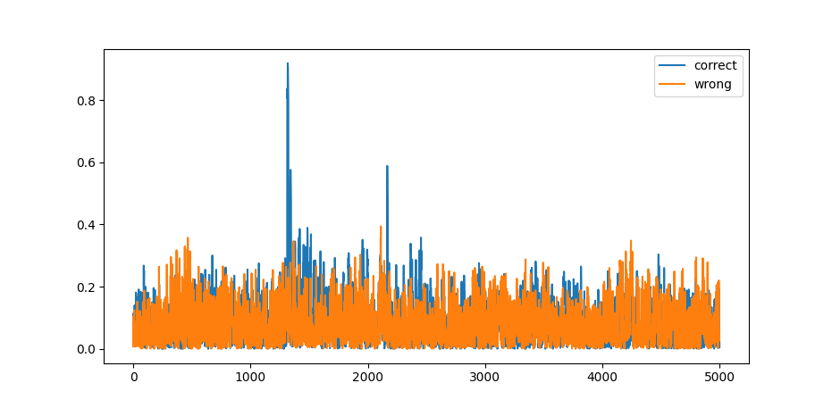
Figure 1: A visualization of Pearson Correlation Coefficient for AES
So what does this graph show? You can see that the correlation coefficient remains reasonably consistent for the wrong key. It never goes above \(\sim 0.4\). The graph of the correct key follows the same pattern — never really reaching above \(\sim 0.4\) — except for one or two spikes. At these spikes apparently our model matches the actual power consumption very closely. These spikes are what we are interested in.
So what did we learn?
Determining what key was used is not only possible using leakage models based on differing processor instructions. We can also correlate memory-based leakage models, using the Hamming Weight or Hamming Distance hypotheses, with multiple power traces to determine how likely it is that a certain memory state occurred during a power trace.