Power Analysis Introductory Walkthrough

What will this course cover?

• Chapter 2 - Installing and configuring capture and analysis tools
• Chapter 3 - Explain Simple Power Analysis by looking at the RSA algorithm
• Chapter 4 - Explain Correlation Power Analysis by looking at the AES algorithm
• Chapter 5 - Setting up tools to compile custom algorithms

IT Security has many fields and layers, all of which aim to investigate how to break and protect the core principles of information security. These principles are confidentiality, integrity and availability¹. One of these fields is Side-Channel analysis. Here the focus lies on how technology interacts with the world around it, and what analysis these interactions can tell us about calculations or operations done by the technology.

One of the techniques within Side-Channel analysis which aims to break confidentiality is Power analysis. Power analysis looks at the power consumption of hardware in order to make statements about the specific calculations done within a computer. Some calculations require a higher amount of power than other calculations.

Take a look at the following picture. If we know that the following Figure 1 records a sequence of two different computations - namely, squaring and taking a product - and we also know that squaring takes marginally less time than taking a product in this case. You could hypothesize where the power trace is taking a product and where the trace is squaring a number.

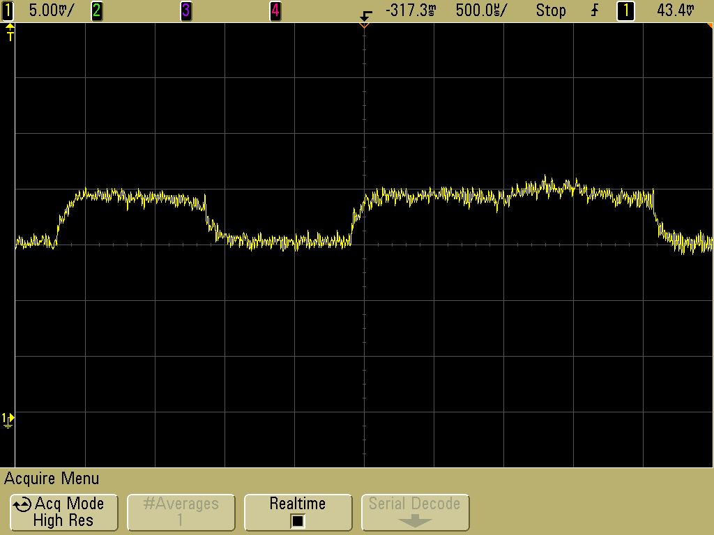
_Figure 1: Power Trace of a RSA encryption by Audriusa (GPFL)

Purpose of this walkthrough

This walkthrough is meant to be an introduction into both power analysis and using the ChipWhisperer framework. It expects you to have some basic knowledge of Python and probably C. It also helps to be comfortable with a terminal and the shell. This walkthrough is not about programming or the shell, however, and most of what is discussed could be followed along with, even if you have very little programming experience. There is, however, a lot of pseudocode.

Furthermore, if you plan on doing your own traces, you will need a ChipWhisperer capturing board. This walkthrough will provide predefined data sets, so you can do some analysis without doing the traces yourself. This could save you from buying a ChipWhisperer capturing board. It is, however, highly recommended doing traces yourself. If you are looking at buying a ChipWhisperer capturing board and don't know what to use, this walkthrough is created using on the CW Lite ARM variant. It is a relatively cheap all-in-one solution.

ChipWhisperer

Normally, to make these power measurements on microprocessors, you need a lot of expensive equipment. Equipment such as multimeters, oscilloscopes, different microcontrollers, connectors, etc. This is where the ChipWhisperer comes in. The ChipWhisperer framework provides microcontrollers to test and run you algorithms on, which are referred to as targets. But also provides measurement devices, which when put together with a target is referred to as a scope. ChipWhisperer goes further than a playground and can be used in real world environments, which makes an ideal framework to learn power analysis with. Partially because scopes can also be connected to other unrelated microprocessors in order to do power measurements on those.

Errors and contributing

This walkthrough along with all the content made for it can be found on GitHub. If you find any errors or feel like something is unclear/left untouched, don't hesitate to create an issue or pull-request on the page there.

Preparing your environment

What will this chapter cover?

• How to install Python and PIP
• How to install dependencies for the ChipWhisperer Python library
• How to install the ChipWhisperer Python library

This chapter expects the reader to have a personal computer (running a modern version of Windows, macOS or a commonly used GNU/Linux distribution) to which one has root/administrator permissions. Furthermore, especially for macOS and GNU/Linux, a basic understanding of the shell is recommended.

Although working with the ChipWhisperer requires little setup, it has some prerequisites. Apart from the usual text editor and Python, we need to install some libraries and toolchains. What we need to install also depends on what we want to achieve with this walkthrough. So the next few sections are going to take you through some common necessities. Along with some of the things that could come in handy whilst following this walkthrough.

Python and PIP

What will this section cover?

• Installing Python
• Installing PIP
• Installing mandatory dependencies: NumPy
• Installing optional dependencies: PyPlot & TQDM

We are going to be heavily relying on Python to do most of our measurements. We are also going to do some data analysis using Python. Because of this heavy reliance on Python, we need to install Python along with some packages for it. Two will be mandatory: NumPy and the ChipWhisperer library (which will be covered in ChipWhisperer) and two are optional but very useful: matplotlib which is used for data plotting and TQDM which is used for visual feedback whilst cracking.

Installing Python

The code provided by this walkthrough uses Python 3 and will NOT work on Python 2. Installing Python is a platform dependent workflow. Here are some common operating systems, for other operating systems a simple Google search or a glance at Python.org should do the trick.

Windows

For Windows, download and run the Windows installer from Python.org. For most people the 64-bit version should be the one.

macOS

For macOS, you can either install Python using Homebrew with the following shell command.

brew install python3

Or you can install Python via the macOS Installer. Depending on whether you own an Intel-based macOS device or an ARM-based macOS, you can select the 64-bit Intel or 64-bit universal2 installer, respectively.

Note: Python on macOS tends to give a lot of problems. There is a big chance that Python is already installed or that only Python 2 is installed.

GNU/Linux

For Debian based systems, including Ubuntu, you can use the following commands.

sudo apt-get update
sudo apt-get install python3 python3-pip

For ArchLinux based systems, including Manjaro, you can use the following command.

sudo pacman -S python python-pip

Validating your installation

To check whether your installation was successful, restart your shell and run the following command.

python3 --version

For most installations, this should have also installed pip. We can verify this with.

pip3 help

Note: If pip is not installing by default when you install Python. A simple google search should do the trick.

NumPy

One of the most common packages used in Python is the NumPy package. We are also going to be using it here to do some data transformations. To install NumPy we can use pip.

pip install numpy

PyPlot

With our data it may be handy to plot our data. Most of the plotting done in this walkthrough has the image attached with it, however. Matplotlib is therefore recommended, but optional. Installing is also via pip.

python -m pip install -U matplotlib

TQDM

To have a better overview of the progress our calculations are making, this walkthrough uses the progress bars from TQDM. This is also optional, but indeed very handy. Installation can be done via pip.

pip install tqdm

Verifying installation of packages

Go into the Python interpreter by running python3 in your shell. We can verify the installation of all the packages by running the following few commands:

import numpy
import matplotlib
import tqdm

If none of those three returned an error, everything is installed correctly!

We have now installed Python, PIP and some packages used throughout this walkthrough. We have also verified that everything is properly installed.

ChipWhisperer

What will this section cover?

• Installing the ChipWhisperer Python Library for different Operating Systems
  • Windows
  • macOS
  • GNU/Linux
• Verifying that the installation was successful

The ChipWhisperer framework has a Python library to interact with its devices. This library is definitely a necessity if you plan on doing your own traces.

Installing the dependencies

The ChipWhisperer python library has some dependencies. Mainly, these dependencies are libusb and make. Let us go over the different operating systems and what needs to be done there.

Note: If something here is not working correctly or not up to date. Refer back to the original ChipWhisperer documentation that can be found here.

Windows

For Windows, we mainly need to install make. There are multiple ways to do this. I suggest installing MinGW and adding MinGW\msys\1.0\bin to your PATH environment variable.

macOS

For macOS, make should already be installed. To install libusb, we can use Homebrew.

brew install libusb

GNU/Linux

For Debian based systems, including Ubuntu, we can install both make and libusb using the following command.

sudo apt install libusb-dev make

For ArchLinux based systems, including Manjaro, we can install both make and libusb using the following command.

sudo pacman -S libusb make

Installing the python library

To install the ChipWhisperer library, we can use pip. We install it with the following command.

pip install chipwhisperer

Linux udev rules

When we are going to start doing traces, one might run into a missing permissions error on Linux. This has to do with the udev rules. How to solve this, refer to the ChipWhisperer docs. This should solve having to run everything with sudo, which is not preferred.

Verifying installation

To verify that the installation succeeded, we can start Python in interactive mode using the python3 shell command. Then we should see something such as the following.

Type "help", "copyright", "credits" or "license" for more information.
>>>

We can use the following Python code to attempt to import the ChipWhisperer python library.

import chipwhisperer

If there aren't any error messages, we have successfully installed the ChipWhisperer python library!

We have now correctly installed everything necessary to perform our own power measurements using ChipWhisperer boards. Furthermore, we have also verified our installation.

A case study: RSA

What will this section cover?

• What is Simple Power Analysis?
• What is the RSA algorithm?
• How can you break implementations of RSA using Simple Power Analysis?

RSA is an encryption algorithm that is used all over the place. That little padlock in your browser; it is powered by RSA. Coding an implementation of RSA is reasonably simple, but the mathematics behind it can prove to be really though. Luckily, there is no need to dive too much into the mathematics to crack RSA using Simple Power analysis. In the chapter on AES, we will go a bit deeper into cache-based Power analysis attacks, why they work exactly and how to perform them on the ChipWhisperer. This chapter is going to skip over a few of the specifics to create a better overview of our method and goals.

What is Simple Power Analysis

Simple Power Analysis (also known as SPA) is a way of leaking information from power measurements of a microprocessor. One can imagine that a microprocessor in idle will use less power than a microprocessor running instructions at maximum speed. Similarly, some processor instructions use more power than others or use power at different intervals. If we take a series of power measurements of a microprocessor performing an algorithm, we use therefore possible say something about the instructions that processors performed. The technique of looking at such power measurements and leaking information from them is called Simple Power Analysis.

We are going to exploit this technique with an encryption algorithm called RSA. In some software implementations of RSA, we can leak secret information just by looking at power measurements of the microprocessor.

What is RSA?

RSA is an algorithm used to do asymmetric encryption. This means we have two distinct keys. Most of the time this means we have one key to encrypt plain text to cipher text, one key to decrypt cipher text back to plain text. It is common to have one of these keys be publicly available while the other is kept extremely private. Because of this, it is also called the public and private key cryptography.

RSA uses one simple principle. For encryption with public key \( e \), for every byte of our plain text \(b_i\) we have encrypted byte \( c_i=b_i^e \) modulo some integer \( N \). For decryption with private key \( d \), for every byte of our cipher text \(c_i\) we have encrypted byte \( b_i=c_i^d \) modulo some integer \( N \). The specific relationship between these numbers is not as important for now.

When one learns that usually the minimum key length for the private key is 1024 bits, one might wonder how these computations are actually done on the bare hardware. It turns out that we can interpret modulo exponentiation as repeated multiplication and squaring alternated with modulo division. This is how that works.

If we are given an enormous number \( x \), and we are tasked with the raising it to the 13th power, we might do it as follows:

\[ x^{13} = x^8 \cdot x^4 \cdot x^1 \]

This is part of the method of Modular Exponentiation. Notice that \((13)_{10} = (1101)_2\). There are some ties with powers of 2 here. Thus, we might write a custom power function in Python as the following.

# Custom implementation of pow(x, y)
def custom_pow(x, y):
    res = 1

    # Until we have reached the highest power
    while (y > 0):
        # If the last byte is a one
        if (y & 0x01):
            res *= x

        # Move on to the next byte
        y >>= 1
        x *= x

    return res

If we add a modulo into our function, we have essentially created a function to do RSA encryption. This is also often how the pseudocode for lower level implementation looks like.

# Custom implementation of pow(x, y) % p
# With p >= 2
def custom_pow_mod(x, y, p):
    res = 1

    # Until we have reached the highest power
    while (y > 0):
        # If the last byte is a one
        if (y & 0x01):
            res *= x
            res %= p # Make sure we stay modulo p

        # Move on to the next byte
        y >>= 1
        x *= x
        x %= p # Make sure we stay modulo p

    return res

Note: This is in fact also how most arbitrary precision library implement raising to the power. This is due to the (relatively) low maximum complexity of this calculation.

If you are already a small bit familiar with Side-Channel Analysis and Power Analysis, you might immediately see what is going wrong here. If you don't see it immediately, let us go through it together.

When we do Power Analysis, we get the power consumption of a microprocessor for a given amount of time. Let us say we would have a computer which purely executing the computation for custom_pow_mod(3, 5, 15). The steps that are taken in this computation are done noted below. Take a look at that the computation and verify it in your head.

custom_pow_mod(3, 5, 15):

res := 1

# Round 1

# [A]
y > 0 = 5 > 0 is true, thus:
    y & 0x01 = 5 & 0x01 is 1, which equals true, thus:
        # [B]
        res := res * x = 1 * 5 = 5
        res := res % 15 = 5 % 15 = 5

    # [C]
    y := y >> 1 = 5 >> 1 = 2
    x := x * x = 3 * 3 = 9
    x := x % 15 = 9 % 15 = 9


# Round 2

# [D]
y > 0 = 2 > 0 is true, thus:
    y & 0x01 = 2 & 0x01 is 0, which equals false

    # [E]
    y := y >> 1 = 2 >> 1 = 1
    x := x * x = 9 * 9 = 81
    x := x % 15 = 81 % 15 = 6

# Round 3

# [F]
y > 0 = 1 > 0 is true, thus:
    y & 0x01 = 1 & 0x01 is 1, which equals true, thus:
        # [G]
        res := res * x = 5 * 6 = 30
        res := res % 15 = 30 % 15 = 0

    # [H]
    y := y >> 1 = 1 >> 1 = 0
    x := x * x = 6 * 6 = 36
    x := x % 15 = 36 % 15 = 6

# Round 4

# [I]
y > 0 = 0 > 0 is false.

# [J]
Result: 0

One might notice that not every round contains the same amount of steps, and thus, we might imagine that the power consumption of our machine looks similar to Figure 1.

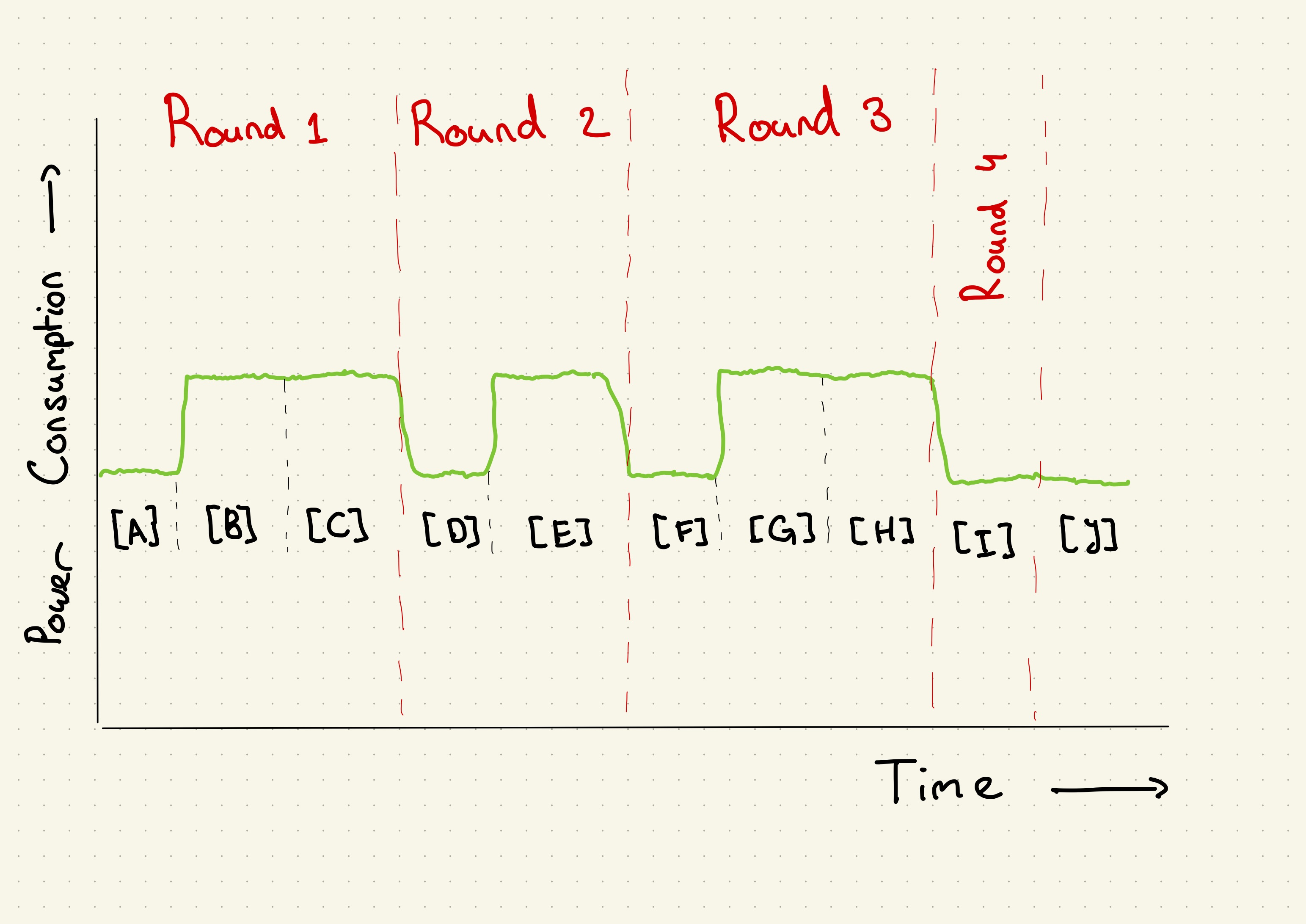
Figure 1: A projected power trace for the custom_pow_mod(3, 5, 15) function call.

Note: This sketch uses the estimate that conditionals and loops (if and while) are less power consuming than normal numerical calculations (>>, * and %), which isn't trivially true, but for the sake of simplicity we are going to assume it is true.

You might notice that given this sketch, we can reconstruct some information about the argument y provided to the custom_pow_mod function. We start with a long spike, thus, the binary number representation of y starts with a 1. This is followed by a short spike, which indicates a 0. And lastly, we see a long spike again. Therefore, we end with an 1. And we get the binary number 101 for our y. This equals 5 in decimal, which is correct.

Let us do another one, now without knowing the answer beforehand. Take a look at Figure 2.

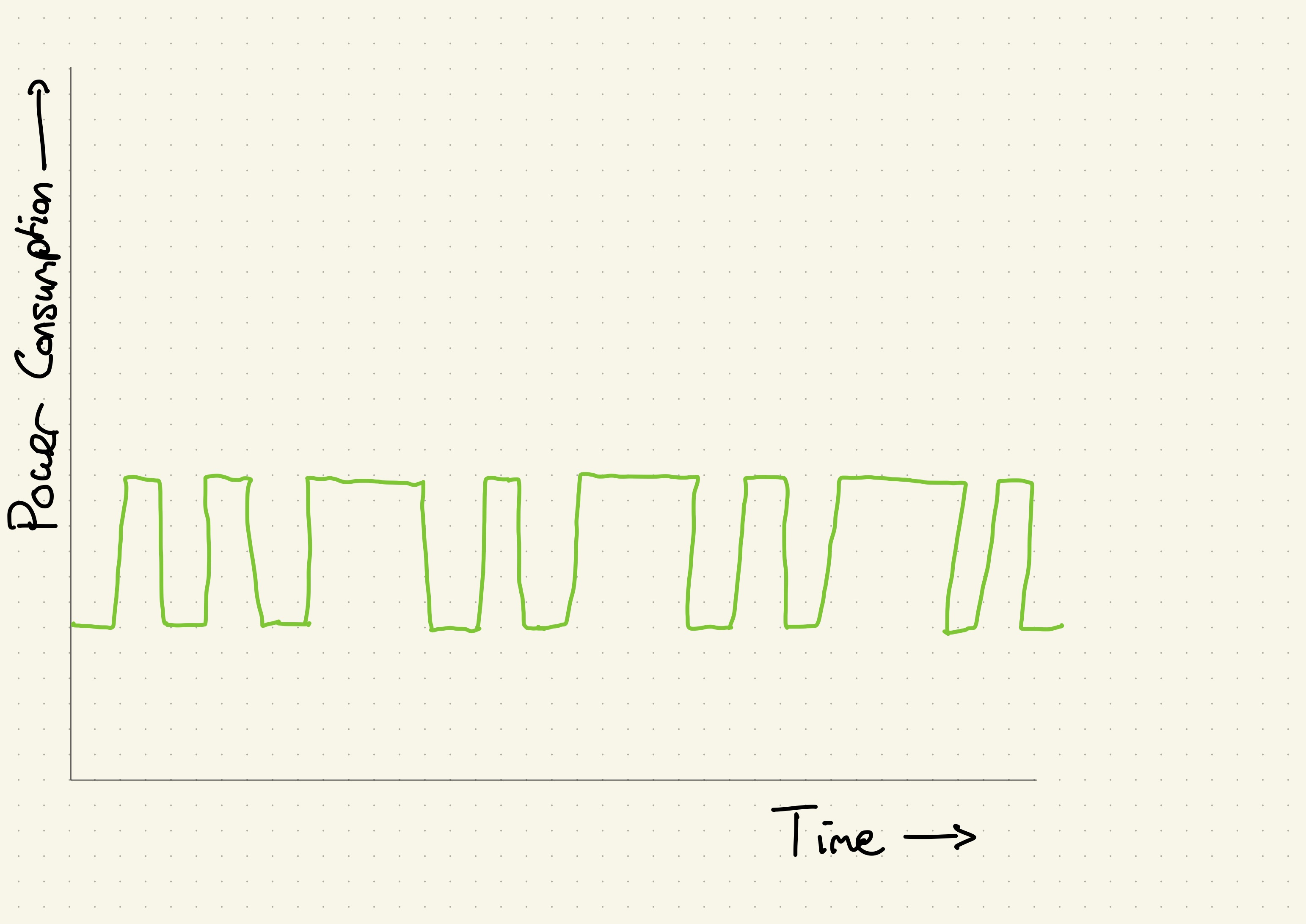
Figure 2: A projected power trace for the custom_pow_mod function.

We start with two short spikes, and thus we start with two zeros. Then we alternate a long spike with a short spike three times. This means we get 00101010. This is equal to decimal 42. And thus the y we started with is 42.

What does this tell us?

The previous code example may seem cherry-picked. In fact, it is not. This code snippet does, however, indicate the concept of Power analysis very nicely and is therefore a fantastic visual example of how to break an RSA implementation. Code following the same principle or even this exact algorithm is extremely common. This means that whilst this exact method may not be applicable everywhere, the underlying idea still is.

So whilst this method specifically is interesting, we are more interested in whether looking into an algorithm can tell us something about data used from the patterns in a power trace. In the next chapter, we are going through how this can be done with AES.

Breaking AES

What will this chapter cover?

• Describe what Correlation Power Analysis is
• Explain in full detail how AES works
• Explain creating a leakage model for AES in full detail
• Cover how to capture multiple traces with the ChipWhisperer framework
• Explain how to crack individual key-bytes from power traces
• Describe in which way we can automate the cracking process and crack whole keys

AES or the Advanced Encryption Standard, is one of the most used symmetric encryption algorithms in today's world. It is used for most encrypted conversations between computers or applications. It is used by your chat apps and by your password manager. AES has the advantage of being relatively fast and easy to understand.

Since AES is very widely used, any found vulnerability should be taken extremely serious. It is widely considered that AES is mathematically secure and therefore perfect implementations of the algorithms should not be vulnerable to most standard attacks. You may see a caveat here:

Have we created perfect implementations of the AES algorithm?

Although there are some AES implementations that have existed for over 2 decades¹. There are still regular updates to these libraries, because from time to time people find new mistakes in the implementation of these algorithms. Code is messy, people make mistakes or are ignorant. Side-Channel analysis is an attack-vector that is often overlooked or ignored since it requires physical access to the device.

In this section we will have a look at how AES works, cracking a naive implementation of the algorithm and see how Power Analysis can be used to expose the key used.

Correlation Power Analysis

What will this section cover?

• Seeing electronics as capacitors
• Hamming Weight and Hamming Distance models
• Correlation coefficients

Not all algorithms perform different processor-instructions based on what (private) key was used. Most symmetric encryption algorithms use some form of byte shuffles and substitution boxes, which have the same amount of processor-instructions for every possible key. Still however, there is a way to crack the keys used by these algorithms using power analysis. The method does not depend on differing instructions, however. Instead, this method focuses on the power used by the memory and registers.

Leakage Models

Power analysis depends on leakage models. These are models which predict how much power is going to be used depending on some task a microprocessor-controlled device performs. In the case of RSA this leakage model was based on the processor instructions. There are other leakage models, however. Correlation Power Analysis is a technique which (most of the time) is memory-based. Within this technique, we try to find out whether there is a connection between our leakage model — and its hypothetical key — and the actual power consumption. Such a connection is also known as a statistical correlation. Memory-based leakage models often choose between two different techniques: Hamming Weight and Hamming Distance. In short: Looking at how much power it would take to set memory is known as the Hamming Distance model. Looking at how much power it would take to maintain memory, which is known as the Hamming Weight model.

Hamming Weight

The Hamming Weight model states that there should be a correlation between the amount of bits in the on or \(1\) state and the amount of power a device uses. This idea stems from the fact that bits in RAM are physical capacitors, which need to be refreshed often. This process of refreshing the state of RAM costs an amount of power which is proportional to the amount of bits in the on or \(1\) state.

For example, the bit-string \(s=010010101\) has \(4\) bits in the in on state and thus the Hamming Weight of \(s\) is \(4\). A general mathematical expression for the Hamming Weight of a bit-string \(s\) is \[ \text{HammingWeight} ( s ) = \# \{s_i \in s : s_i = 1\} \]

Hamming Distance

The Hamming Distance model states that there should be a correlation between the amount of bits switching between the on (\(1\)) and the off (\(0\)) state and the amount of power a device uses. Register bits are often set to a specific voltage before reassignment. This is for power efficiency reasons. Because of this the Hamming Distance model works better on hardware implementations of encryption algorithms.

For example, switching from the bit-string \(p=010010101\) to \(c=110011001\) yields a Hamming Distance of \(3\), because \(3\) bits were flipped. A general mathematical expression for the Hamming Distance from a bit-string \(p\) to a bit-string \(c\) with \(|p| = |c|\) is \[ \text{HammingDistance} ( p, c ) = \# \{ i : p_i \not= c_i \text{ with } i \in \{1,...,|p|\} \} \]

Memory-based models

Now that we have seen two different models for correlation between memory-usage and power consumption, we might ask ourselves how we go from these concepts to a functional model for an encryption algorithm. We have to determine a memory state which we can test for. Trivially, this memory state should be dependent on the (private) key used. Next to that, we have two preferences for this memory state:

1. Ideally, the memory state is dependent on the input string. This allows us to look for different memory values. Instead of just searching for the same derivative of the key memory value.
2. Preferably, the Hamming Weight/Distance value holds for a longer time. With Hamming Weight, for example, a memory state just before shifting bytes around works better, because transpositions don't affect the Hamming Weight.

Correlations

In order to determine whether there is a connection between a leakage model and the power consumption, we are going to be determining whether there is a correlation between that leakage model and the power trace at every point in time. This means we are going to need multiple power traces: multiple power consumption values for each point in time. This assumes we have already (roughly) synchronized our power traces. On the ChipWhisperer, this done on the instruction level with our compiled algorithms, so we don't have to worry about it too much.

Pearson Correlation Coefficients

Now, however, we are also tasked with determining how well our set of power traces correlates with our leakage model. Just to summarize, we want to know how likely it is that our modeled power usage has a similar pattern to the actual power usage. In statistics this is known as the modeled power usage and the actual power usage having a high correlation. If two functions are in perfect correlation, both functions rise and fall at the same time.

This is what the Pearson correlation coefficient indicates. We provide it with two functions or arrays, and it will give us a value between \(-1\) and \(1\), indicating whether the two functions correlate. \(1\) meaning extreme but almost unrealistic levels of correlation, \(0\) meaning no correlation and \(-1\) meaning an inverse correlation. How the Pearson correlation coefficient manages to do this is not as important for us, but reading the Wikipedia page can be very interesting. What is important for us now, is the formula so we can use it in our code.

\[ \rho_{X,Y} = \frac{\text{cov}(X,Y)}{\sigma_X \sigma_Y} \]

This may not be entirely clear to most people without knowledge of statistics. So let us break it down.

• \(\rho\) is the letter commonly used to represent the Pearson correlation coefficient.
• \(X\) and \(Y\) are our functions and can actually be represented as a finite list of numbers in our case. This means \(X = \{ x_0, \ldots, x_n \}\) and \(Y = \{ y_0, \ldots, y_n \}\) with \(n\) being an integer greater than zero.
• \(\text{cov}(X,Y)\) is the covariance of \(X\) and \(Y\). This can be calculated with \(\text{cov}(X,Y)=\mathbb{E}[(X - \mu_X)(Y - \mu_Y)] = \frac{1}{n} \sum_{i=0}^n (x_i - \mu_X)(y_i - \mu_Y) \), with \(\mu_X\) and \(\mu_Y\) being the mean of \(X\) and \(Y\), respectively.
• \(\sigma_X\) and \(\sigma_Y\) being the standard deviation of \(X\) and \(Y\), respectively. The standard deviation can be calculated with \(\sigma_X = \sqrt{\frac{1}{n} \sum_{i=0}^n (x_i - \mu_X)^2}\) with \(\mu_X\) being the mean of \(X\).

So let us try to visualize what is actually going to be happening.

We are calculating all the correlation coefficients between the power traces and our leakage model for all the points in time. Then we choose the highest correlation coefficient. At that point in time our hypothetical memory state should have occurred. When we repeat this with all keys in our leakage model, the correct key should correlate most at some point in the power trace.

For example, if we take 100 power traces and correlate each point of time with a memory-based leakage model. Once using the correct key, and another time using a wrong key. It might look something like the following graph. On the vertical axis is the absolute of the correlation and on the horizontal axis we see time represented by \(5000\) power measurements.

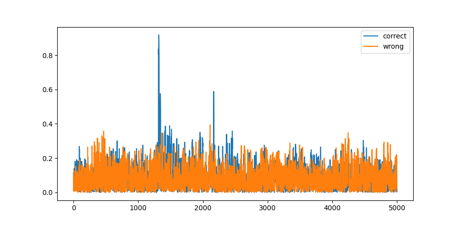
Figure 1: A visualization of Pearson Correlation Coefficient for AES

So what does this graph show? You can see that the correlation coefficient remains reasonably consistent for the wrong key. It never goes above \(\sim 0.4\). The graph of the correct key follows the same pattern — never really reaching above \(\sim 0.4\) — except for one or two spikes. At these spikes apparently our model matches the actual power consumption very closely. These spikes are what we are interested in.

So what did we learn?

Determining what key was used is not only possible using leakage models based on differing processor instructions. We can also correlate memory-based leakage models, using the Hamming Weight or Hamming Distance hypotheses, with multiple power traces to determine how likely it is that a certain memory state occurred during a power trace.

How AES Works

What will this section cover?

• The inner workings of the AES algorithm.
• Different operations utilized by Rijndael block ciphers:
  • XOR operations
  • Byte subtitutions and S-Boxes
  • Shifting of Rows
  • Mixing of Rows

In order to do break AES with power analysis, we need a reasonably detailed understanding of how AES works. So let us do a crash course.

The AES algorithm is a subset of the Rijndael block cipher algorithm and has basically become synonymous with it. As the name Rijndael block cipher implies, we apply the encryption to fixed-size blocks of plain text. With the size of the blocks being equal to the key size. The encryption is based on alternating XOR operations and shuffling the bytes of the blocks. Let dive into each individual component of the algorithm.

The Plan

As said previously, the AES algorithm works by alternating XOR operations with the shuffling of the bytes of the blocks. The algorithm specifies that this is done in rounds. Since AES has 3 different key sizes (128, 192 and 256 bits), each different key size also has a different number of rounds. The amount of rounds are 10, 12, and 14, respectively.

How does a round look like? Although the first round and the last round have small differences to the rest we can divide all the rounds up into two sections the shuffling of bytes and the XOR operation. Let us first have a look at the XOR operations.

XOR operations

The XOR operation is essentially the mixing in of the key and is what makes the running of the AES algorithm different depending on what key is used. Firstly, in order to make reversal even more different, we create multiple new keys from the original key. This is called the AES key schedule. This walkthrough will not go into detail on how this key-expansion works, but if interested one can look up details. The part which is important to this walkthrough is that after this expansion we have as many new keys as we have rounds. We will number all the keys to form \(k_0\) to \(k_{10}\) (assuming we are using 128 bit AES). Here \(k_0\) is the original key and \(k_1\) till \(k_{10}\) are the expanded keys.

Figure 1: The AES Key Schedule

With these keys we perform a XOR on a block. The XOR operation is a notorious one way operation. This is due to the lack of information the output shares about the input. When we do a one bit XOR operation, and we receive 1 as an output, the input could have been (0,1) or (1,0). We also have two options when we get 0 as output. In the case of one bit, this is not that useful. However, when we have a lot of bits the XOR operator is impossible to instantly reverse for every output and brute forcing time is equal to trying every option divided by two. Mathematically this caused by the XOR operation being non-injective. When we have the outcome and one of the inputs however, this step is extremely easy to reverse. These two properties make it ideal for a lot of encryption algorithms.

Figure 2: The non-injective nature of the XOR operation

Shuffling of bytes

Next let us have a look at the other parts of each round. The shuffling of the block bytes. Rijndael block ciphers have 3 distinct shuffling techniques: substitution, shifting, and mixing. We are going to have a look at all three of these shuffling techniques, but let us first have a look at how Rijndael block ciphers view each block.

Block-of-blocks?

Rijndael looks at blocks as a matrix of bytes. For the key sizes of key sizes of 128, 192 and 256 bits, we have 4 by 4, 6 by 6 and 8 by 8 matrices, respectively. This would mean that a 128-bit key with bytes \(b_0, ..., b_{15}\) is turned into \[ \begin{bmatrix} b_0 & b_4 & b_8 & b_{12} \\ b_1 & b_5 & b_9 & b_{13} \\ b_2 & b_6 & b_{10} & b_{14} \\ b_3 & b_7 & b_{11} & b_{15} \end{bmatrix} \] Turning a long string of bytes into a matrix allows for matrix operations, which are common operations for computers. This provides both clarity and speed.

Substitution

Now comes one of the most genius but strange parts of the Rijndael block cipher. This is the substitution box. A substitution box is basically a lookup table to replace (or substitute) a byte with the one from the lookup table. Some demands for such a lookup table (when used in encryption algorithms) may be:

• Reversible: In order to find back the original byte, we want to be able to reverse the process.
• Non-Linear: In order to make resistant to linear and differential cryptanalysis, the lookup should be very difficult to approximate with a linear function.
• Fixed Output Sizing: In order to reduce the complexity and loss of excess data, we want to output to have a fixed bit size (preferably the same as the input).

The Rijndael S-Box does all these things. Since it has all of these properties, how it specifically looks is not important. Every implementation of AES can save the Substitution-Box and its inverse in static memory since it is public knowledge.

Here is the Rijndael S-Box as a Python array.

# Rijndael Substitution box
SBox = [
    # 0    1    2    3    4    5    6    7    8    9    a    b    c    d    e    f
    0x63,0x7c,0x77,0x7b,0xf2,0x6b,0x6f,0xc5,0x30,0x01,0x67,0x2b,0xfe,0xd7,0xab,0x76, # 0
    0xca,0x82,0xc9,0x7d,0xfa,0x59,0x47,0xf0,0xad,0xd4,0xa2,0xaf,0x9c,0xa4,0x72,0xc0, # 1
    0xb7,0xfd,0x93,0x26,0x36,0x3f,0xf7,0xcc,0x34,0xa5,0xe5,0xf1,0x71,0xd8,0x31,0x15, # 2
    0x04,0xc7,0x23,0xc3,0x18,0x96,0x05,0x9a,0x07,0x12,0x80,0xe2,0xeb,0x27,0xb2,0x75, # 3
    0x09,0x83,0x2c,0x1a,0x1b,0x6e,0x5a,0xa0,0x52,0x3b,0xd6,0xb3,0x29,0xe3,0x2f,0x84, # 4
    0x53,0xd1,0x00,0xed,0x20,0xfc,0xb1,0x5b,0x6a,0xcb,0xbe,0x39,0x4a,0x4c,0x58,0xcf, # 5
    0xd0,0xef,0xaa,0xfb,0x43,0x4d,0x33,0x85,0x45,0xf9,0x02,0x7f,0x50,0x3c,0x9f,0xa8, # 6
    0x51,0xa3,0x40,0x8f,0x92,0x9d,0x38,0xf5,0xbc,0xb6,0xda,0x21,0x10,0xff,0xf3,0xd2, # 7
    0xcd,0x0c,0x13,0xec,0x5f,0x97,0x44,0x17,0xc4,0xa7,0x7e,0x3d,0x64,0x5d,0x19,0x73, # 8
    0x60,0x81,0x4f,0xdc,0x22,0x2a,0x90,0x88,0x46,0xee,0xb8,0x14,0xde,0x5e,0x0b,0xdb, # 9
    0xe0,0x32,0x3a,0x0a,0x49,0x06,0x24,0x5c,0xc2,0xd3,0xac,0x62,0x91,0x95,0xe4,0x79, # a
    0xe7,0xc8,0x37,0x6d,0x8d,0xd5,0x4e,0xa9,0x6c,0x56,0xf4,0xea,0x65,0x7a,0xae,0x08, # b
    0xba,0x78,0x25,0x2e,0x1c,0xa6,0xb4,0xc6,0xe8,0xdd,0x74,0x1f,0x4b,0xbd,0x8b,0x8a, # c
    0x70,0x3e,0xb5,0x66,0x48,0x03,0xf6,0x0e,0x61,0x35,0x57,0xb9,0x86,0xc1,0x1d,0x9e, # d
    0xe1,0xf8,0x98,0x11,0x69,0xd9,0x8e,0x94,0x9b,0x1e,0x87,0xe9,0xce,0x55,0x28,0xdf, # e
    0x8c,0xa1,0x89,0x0d,0xbf,0xe6,0x42,0x68,0x41,0x99,0x2d,0x0f,0xb0,0x54,0xbb,0x16  # f
]

Shifting

The most plain, but equally important, round step is the shifting of the rows. This step prevents the columns (4 consecutive bytes in the case of the 128 bit variant) from being encrypted and decrypted separately. The step consists of shifting the first row of the matrix by zero, the second by one, the third by two and the fourth by three spaces. This is depicted in Figure 3.

Figure 3: Rijndael block cipher's Shift Row

Mixing

The last shuffling step mixes the columns in order to create cryptographic diffusion, which makes it resistant to statistical analysis attacks. The step works by multiplying each column with the following invertible matrix (multiplication meaning modulo multiplication and addition meaning XOR): \[ \begin{bmatrix} 2 & 3 & 1 & 1 \\ 1 & 2 & 3 & 1 \\ 1 & 1 & 2 & 3 \\ 3 & 1 & 1 & 2 \end{bmatrix} \]

Overview

Let us now provide an overview for how a typical AES encryption looks. One can imagine that the decryption is just the inverse of these actions we will therefore gloss over that part.

As said before, the AES encryption process works in rounds. With every round needing a separate expanded key. Therefore, the first step is to create these key expansions as described in XOR Operations. Immediately following this we that the initial round key \(k_0\) and apply the XOR with it to each block.

After the summation with the initial round key we will start applying rounds (9, 11 and 13 rounds for key sizes 128, 192 and 256 bits, respectively). These rounds apply steps in the following order: Firstly, we do a substitution with the Rijndael S-Box. Secondly, we shift the rows of the matrix. Thirdly, we mix the columns of the matrix up. Lastly, we add the round key for that round.

If you are counting along, you will notice that the final round is missing. This is because the final round is a little different. The only difference being that we skip the mixing of columns step, since it serves no purpose in the final round.

This all results in the following process:

1. Key Expansion
2. Apply \(k_0\) by XOR
3. Apply 9, 11, or 13 rounds
   1. Substitution with the Rijndael S-Box
   2. Shift the rows
   3. Mix the columns
   4. Apply \(k_n\) by XOR with \(n\) being the round number
4. Final round
   1. Substitution with the Rijndael S-Box
   2. Shift the rows
   3. Apply \(k_n\) by XOR with \(n\) being the round number

After reading this section should have a basic overview and understanding of how AES works, which you will need for your Power analysis. If you want a more visual explanation of the AES algorithm, you could watch AES Explained by Computerphile.

Modeling AES

What will this section cover?

• Creating a leakage model for AES
• Implementing a leakage model for AES in Python

In order to make sensible statements about the power usage of AES, we are going to make a leakage model of the AES algorithm. To do this, we need some to determine the optimal memory state to target. When we have determined that state, we are going to implement that leakage model in Python.

Hamming Distance and Hamming Weight

Remember that we covered both the Hamming Distance and Hamming Weight hypotheses of looking at memory-based leakage model in Correlation Power Analysis. In this walkthrough, we are going to go through a software implementation of AES. The .hex file of the algorithm for ChipWhisperer targets can be found here. Since we are using a software implementation, this walkthrough is going to focus on the Hamming Weight-based leakage model.

We can easily calculate Hamming Weight with the following lambda function.

HammingWeightFn = lambda x: bin(x).count('1')

Although it can be worth it to save this to memory, to speed to computation time later on.

# Precompute Hamming Weight
HammingWeight = [ HammingWeightFn(n) for n in range (0x00, 0xff + 1) ] 

Finding a memory state

Suppose we have an input block Input and an output block Output, which is a reasonably common situation. If we wanted to check whether a supposed Key is the key used, we could run through the entire algorithm to check whether \(\text{AES}(Input, Key) = Output\). This is quite inefficient and is no better than brute forcing the key. Knowing what we know about the memory state of AES, we can however do two extreme optimizations.

Shortcutting calculations

The first optimization we can do has to do with identifying the first memory state where the key and the Input are combined. If we can identify this memory state in the power trace, we can determine a probability a certain key was used. There are two problems with this, however. Firstly, identifying the presence or the location of this memory state is non-trivial. It is very difficult to manually look at a power trace and tell something about memory states. This is mostly due to the variances in baseline power consumption but also due to noise and other factors. Some of these factors however can be nullified if we look at multiple power traces instead of one. In order to make it even easier, we also look at different input blocks. This allows us to shortcut calculation time by a lot, since we don't have to do multiple rounds. But we still have to brute force through every key option.

Limiting the amount of keys

If we have done the first optimization, there is another optimization which would lower the amount of possible keys. For the 128 (\(2^{128}\) different keys), 192 (\(2^{192}\) different keys) and 256 (\(2^{256}\) different keys) bits key variants, this leaves just \(2^{12}\), \((3 \cdot 2^{11})\) and \(2^{13}\) key possibilities left, respectively. These are massive differences, which allows us to break AES in just a few seconds.

How does it work? Please read back How AES Works - Shifting for one second and see if you find what we can exploit, when have a value before this step happens. As it mentions this, the step is needed to prevent attacking each column individually. Since we can now produce a value before this step is done. We can attempt to break parts of the key one at the time. The parts of this key are called sub-keys, and they are 1 byte in size. This means we can take the sum of different values for the sub-keys instead of the product.

Putting this together

Let us make a model of the memory states power usage. This model should provide us with a number that should correlate with the power traces at the point of which this first SBox step is done. This leaves us with a longstanding memory state which is dependent on both the key and the input string. Two items we both preferred for our leakage model as explained in Memory-based models. The Python code for performing our model on a single byte input string using a single byte from the key (also called a sub-key) is the following.

def hypothetical_power_usage(subkey, plain_text_char):

    # Use the Hamming Weight power usage model
    return HammingWeight[

        # Do a SBox look up of the XOR-ed value
        #
        # Since the Hamming Weight of the SBox value will
        # persist for longer in memory this will make finding the
        # pattern easier. It is also still before the Row Shifting
        # so it doesn't cause trouble.
        SBox [

            # The initial round key XOR-ed with the plain text
            subkey ^ plain_text_char
        ]
    ]

Capture multiple traces

What will this section cover?

• Setting up our ChipWhisperer scope and target
• Running AES on our ChipWhisperer target
• Performing a power trace of our algorithm
• Saving multiple power traces to a file

Cracking the key used by AES with Power Analysis is a lot more complex than was the case with RSA. Looking at one trace of an RSA decryption can potentially give you all the information you need to crack the private key. With AES and, more generally, with Correlation Power Analysis, it is necessary to perform multiple traces and average those power traces out. In this section, we are going to have a look at how we can set up a ChipWhisperer to measure power traces. Afterwards, we are going to do some traces and learn how to save them, so we can later do more detailed analysis on them.

Note: If you just want to move on with the analysis or don't have a ChipWhisperer board at hand, you can download a pre-made power trace over here.

Setting up our ChipWhisperer board

Assuming that you have correctly set up your software environment, we can start connecting and setting up our ChipWhisperer board. This is going to go in 2 steps:

1. Fetching and setting up our scope
2. Setting up and programming our target

Basics

Before we actually start scripting, we are starting in the Python Interpreter. We can get into the Python Interpreter from our shell using the following command:

python3

In order to then get started with the ChipWhisperer Python Library, we can import the library with:

import chipwhisperer as cw

If one gets an error here, verify that the ChipWhisperer Python library is properly installed. Otherwise, we can try to connect our ChipWhisperer Capture board to our computer via USB and run the following command to connect to the Capture board.

scope = cw.scope()

This should connect to our capture board. On some ChipWhisperer capture boards an extra light might start flickering. If you get an error, there most probably is something wrong with your connection. If you are on Linux, perhaps you have to set up some udev rules.

Now we are going to set some settings used by the ChipWhisperer board(s). For now, we will just use the default settings. That works well enough for now, but if you want an overview of the possible settings, look over here. We can select the default settings using the following command.

scope.default_setup()

Then we have to fetch the target board. This is going to contain all the connections and settings about the microprocessor which is going to execute our algorithm. If you have hooked up your target — this is done automatically for the ChipWhisperer Lite boards — you can use the following command to fetch the target object.

target = cw.target(scope)

Now in order to safely disconnect our target and capture board, and we can use the following two commands.

scope.disconnect()
target.disconnect()

Now we know the basics of how to set up and interact with the connection between our computer and the ChipWhisperer board.

Scripting

We know some basic commands, so we can actually start scripting. We create a Python file, and put the basic commands — we just learned — into it.

This is what it will look like.

import chipwhisperer as cw

# Setup a connection with the CW board
# and fetch the scope for using this board.
scope = cw.scope()

# The default settings are fine for now.
scope.default_setup()

# Fetch the target from the scope
# This should be automatically connected
target = cw.target(scope)

#
# We do our logic here!
#

scope.dis()
target.dis()

Running this script using the python3 file-name.py command should work just fine and now we can start actually working with an encryption algorithm.

Uploading the algorithm source code

Depending on what target we are using, we need to upload different software. We can compile this software ourselves, but a lot of compiled code can also be found online. The compiled code for AES can be found here.

Note: This walkthrough will demonstrate the process of uploading source code for the ChipWhisperer Lite ARM board, although many of the concepts here can also be applied to other boards. More information on other uploading source code for other targets can be found here.

In order to upload a binary to the CW Lite ARM, we will use the Intel Hex format. Therefore, assuming we are using the ChipWhisperer Lite 32-bit ARM-edition, we can the CWLITEARM hex file provided in the SimpleSerial AES GitHub folder. Assuming we have downloaded that .hex file and put it into a folder called hexfiles we can use the following Python code to upload the program to our target.

# ... Connecting to the scope / target

from chipwhisperer.capture.api.programmers import STM32FProgrammer
import os

# Initiate a new STM32F Program
# STM32 being the ARM microcontroller that we are using
# https://en.wikipedia.org/wiki/STM32#STM32_F3
program = STM32FProgrammer

# Get the path to the current folder
# Adjust accordingly
aes_firmware_dir = os.path.dirname(os.path.realpath(__file__))
aes_hex_path = os.path.join(aes_firmware_dir, r"hexfiles/simpleserial-aes-CWLITEARM.hex")

# Apply the program to the actual target
# This allows us to run the hex code on the microcontroller
cw.program_target(scope, program, aes_hex_path)

# ... Disconnecting from the scope / target

Now that we have uploaded our program to the ChipWhisperer target board, we start capturing traces.

Capturing a trace

In order to run our first trace, we need a key and some plain text. The program we are using is based on 128-bit AES, and, therefore, we should provide a 128-bit key and a multiple or 128 bits for our plain text. We can quite easily create our first trace, with the following code.

# Define the key used for the encryption
# This key has to be 128 bits = 16 bytes
# = 16 ascii characters in length
key_str = 'H4ck3rm4n-l33t42'

# Convert the key to a byte array
key = bytearray(key_str, 'ascii')

# Define the plain text used
# This plain text has to be a multiple of
# 128 bits = 16 bytes = 16 ascii characters in length.
plain_text = bytearray('a' * 16, 'ascii')

# Capture the actual trace
trace = cw.capture_trace(scope, target, plain_text, key)

NOTE: Within the SimpleSerial protocol — which is used under the hood by the ChipWhisperer devices — the capture_trace function corresponds with a couple of steps (arming the ChipWhisperer, sending the key/plaintext and retrieving the trace data, etc.). This can become important when implementing your own algorithms. There it may be important to replace this one function with its individual steps to get more control over the commands send. This can be seen in the Python code of the SimpleSerial C template.

This is very interesting, but we don't really have any confirmation or visualization. So let us visualize it with matplotlib.

import matplotlib.pyplot as plt

plt.plot(trace.wave)
plt.show()

This should look something like Figure 1.

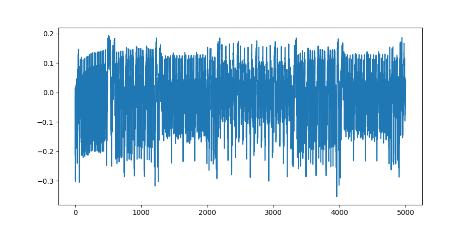
Figure 1: AES Single Power Trace

Capturing more than one trace

We can turn this into multiple traces with a simple for loop. Here we are going to be using the TQDM library to have a nice progress bar. So let us create 100 traces with random input text and save all relevant data into a numpy arrays. This way we can save the eventual traces and plain texts to a file.

First we define a function for creating random plain text strings.

import string
import random

def random_string(length):
    # Define the alphabet of the random string
    # Here we take the lowercase latin alphabet in ascii encoding
    # e.g. "cpjsapcnrsdtjvlo", "btqfocsprbualtwt" or "yzkwewjbkpmriccx"
    alphabet = string.ascii_lowercase

    # Return a string with the given length with randomly chosen chars
    return ''.join(random.choice(alphabet) for i in range(length))

Then we capture some traces.

from tqdm import trange

# Define the key used for the encryption
# This key has to be 128 bits = 16 bytes
# = 16 ascii characters in length
key_str = 'H4ck3rm4n-l33t42'

# Convert the key to a byte array
key = bytearray(key_str, 'ascii')

# Define the constant for the amount of traces
N = 100

textins = []
traces = []

# Loop through all traces
for i in trange(N, desc="Capturing traces"):

    # Define the plain text used
    # This plain text has to be a multiple of
    # 128 bits = 16 bytes = 16 ascii characters in length.
    plain_text = bytearray(random_string(16), 'ascii')

    # Capture the actual trace
    trace = cw.capture_trace(scope, target, plain_text, key)

    # If the capture timed out move to the next capture
    if trace is None:
        continue

    textins.append(plain_text)
    traces.append(trace.wave)

Then we turn this into numpy arrays.

np_traces = np.asarray(traces)
np_textins = np.asarray(textins)

Then we can save it to a file.

np.save('output/traces.npy', np_traces)
np.save('output/textins.npy', np_textins)

This way we can later load it.

For more information on how to do scripting with the ChipWhisperer python module have a look over here. Disclaimer: This is quite heavy.

We have now correctly set up our ChipWhisperer equipment, uploaded the source code of the encryption algorithm we are using to the target, captured power traces of the target and saved those power traces to a file on our system. Now, we are ready to do some analysis on those power traces.

Crack individual key-byte

What will this section cover?

• Loading our saved power traces
• Calculating Pearson correlation coefficients in Python
• Finding the highest Pearson correlation coefficient for a byte of the key used

After creating files containing multiple power traces in the previous section, we can now start analyzing our traces and attempt to crack some bytes with the leakage model we defined in Modeling AES.

So what did we have for our leakage model up until now?

HammingWeightFn = lambda x: bin(x).count('1')

# Precompute Hamming Weight
HammingWeight = [ HammingWeightFn(n) for n in range (0x00, 0xff + 1) ] 

# Rijndael Substitution box
SBox = [
    # 0    1    2    3    4    5    6    7    8    9    a    b    c    d    e    f
    0x63,0x7c,0x77,0x7b,0xf2,0x6b,0x6f,0xc5,0x30,0x01,0x67,0x2b,0xfe,0xd7,0xab,0x76, # 0
    0xca,0x82,0xc9,0x7d,0xfa,0x59,0x47,0xf0,0xad,0xd4,0xa2,0xaf,0x9c,0xa4,0x72,0xc0, # 1
    0xb7,0xfd,0x93,0x26,0x36,0x3f,0xf7,0xcc,0x34,0xa5,0xe5,0xf1,0x71,0xd8,0x31,0x15, # 2
    0x04,0xc7,0x23,0xc3,0x18,0x96,0x05,0x9a,0x07,0x12,0x80,0xe2,0xeb,0x27,0xb2,0x75, # 3
    0x09,0x83,0x2c,0x1a,0x1b,0x6e,0x5a,0xa0,0x52,0x3b,0xd6,0xb3,0x29,0xe3,0x2f,0x84, # 4
    0x53,0xd1,0x00,0xed,0x20,0xfc,0xb1,0x5b,0x6a,0xcb,0xbe,0x39,0x4a,0x4c,0x58,0xcf, # 5
    0xd0,0xef,0xaa,0xfb,0x43,0x4d,0x33,0x85,0x45,0xf9,0x02,0x7f,0x50,0x3c,0x9f,0xa8, # 6
    0x51,0xa3,0x40,0x8f,0x92,0x9d,0x38,0xf5,0xbc,0xb6,0xda,0x21,0x10,0xff,0xf3,0xd2, # 7
    0xcd,0x0c,0x13,0xec,0x5f,0x97,0x44,0x17,0xc4,0xa7,0x7e,0x3d,0x64,0x5d,0x19,0x73, # 8
    0x60,0x81,0x4f,0xdc,0x22,0x2a,0x90,0x88,0x46,0xee,0xb8,0x14,0xde,0x5e,0x0b,0xdb, # 9
    0xe0,0x32,0x3a,0x0a,0x49,0x06,0x24,0x5c,0xc2,0xd3,0xac,0x62,0x91,0x95,0xe4,0x79, # a
    0xe7,0xc8,0x37,0x6d,0x8d,0xd5,0x4e,0xa9,0x6c,0x56,0xf4,0xea,0x65,0x7a,0xae,0x08, # b
    0xba,0x78,0x25,0x2e,0x1c,0xa6,0xb4,0xc6,0xe8,0xdd,0x74,0x1f,0x4b,0xbd,0x8b,0x8a, # c
    0x70,0x3e,0xb5,0x66,0x48,0x03,0xf6,0x0e,0x61,0x35,0x57,0xb9,0x86,0xc1,0x1d,0x9e, # d
    0xe1,0xf8,0x98,0x11,0x69,0xd9,0x8e,0x94,0x9b,0x1e,0x87,0xe9,0xce,0x55,0x28,0xdf, # e
    0x8c,0xa1,0x89,0x0d,0xbf,0xe6,0x42,0x68,0x41,0x99,0x2d,0x0f,0xb0,0x54,0xbb,0x16  # f
]

def hypothetical_power_usage(subkey, plain_text_char):

    # Use the Hamming Weight power usage model
    return HammingWeight[

        # Do a SBox look up of the XOR-ed value
        #
        # Since the Hamming Weight of the SBox value will
        # persist for longer in memory this will make finding the
        # pattern easier. It is also still before the Row Shifting
        # so it doesn't cause trouble.
        SBox [

            # The initial round key XOR-ed with the plain text
            subkey ^ plain_text_char
        ]
    ]

We are going to take this as a starting point of a new Python script. This walkthrough is will refer to that Python file as crack.py. We can thus run this script from our shell using python3 crack.py.

Loading back in our traces

In order to load the power traces we created in the previous section, we can add the follow few lines which will load in the NumPy arrays. The traces here are put into a subfolder called output. If for any reason making power traces did not work out, or you don't own a ChipWhisperer board, but you still want to continue, you can download some pre-made traces from here.

import numpy as np

traces = np.load('output/traces.npy')
textins = np.load('output/textins.npy')

num_traces = np.shape(traces)[0]
num_points = np.shape(traces)[1]

Now we can use our from the traces variable, we know how many traces we have (num_traces), and how many points in time we have per trace (num_points).

Implementing Pearson Correlation Coefficients

As explained in the section on Correlation Power Analysis, we are going to be using Pearson Correlation Coefficients to detect whether our power trace is similar to our leakage model. So let us implement Pearson Correlation Coefficients in Python.

def covariance(X, Y):
    if len(X) != len(Y):
        print("Lengths are unequal, quiting...")
        quit()

    n = len(X)
    mean_x = np.mean(X, dtype=np.float64)
    mean_y = np.mean(Y, dtype=np.float64)

    return np.sum((X - mean_x) * (Y - mean_y)) / n

def standard_deviation(X):
    n = len(X)
    mean_x = np.mean(X, dtype=np.float64)

    return np.sqrt( np.sum( np.power( (X - mean_x), 2 ) ) / n )

def pearson_correlation_coefficient(X, Y):
    cov = covariance(X, Y)
    sd_x = standard_deviation(X)
    sd_y = standard_deviation(Y)

    return cov / ( sd_x * sd_y ) 

Although this code is very inefficient, and does a lot of unnecessary and double calculations, it will serve well for now. We are going to be optimizing this code in Sidenote: optimizing our code.

Cracking a single byte of the key

As explained in Modeling AES, we can — using power analysis — crack the AES key byte by byte. So let us start with a single one. We are going to go through every possibility and see which byte one provides the highest correlation coefficient between the actual power trace and our modeled power usage. The important realization here is that we are doing a correlation between all individual power trace points and the hypothetical power consumption, and we will select the maximum correlation coefficient for all sub-key guesses. This is because we still have no idea where within the power trace the first round actually takes place. If we look at all points of each power trace, the location where the first round takes place should have the highest correlation. We will demonstrate this later on.

from tqdm import trange

def calculate_correlation_coefficients(subkey, subkey_index):
    # Declare a numpy for the hypothetical power usage
    hypothetical_power = np.zeros(num_traces)

    for trace_index in range(0, num_traces):
        hypothetical_power[trace_index] = hypothetical_power_usage(
            subkey,
            textins[trace_index][subkey_index]
        )

    # We are going to the determine correlations between each trace point
    # and the hypothetical power usage. This will save all those coefficients
    point_correlation = np.zeros(num_points)

    # Loop through all points and determine their correlation coefficients
    for point_index in range(0, num_points):
        point_correlation[point_index] = pearson_correlation_coefficient(
            hypothetical_power,

            # Look at the individual traces points for every trace
            traces[:, point_index]
        )

    return point_correlation

# Save all correlation coefficients
max_correlation_coefficients = np.zeros(256)

# Loop through values this subkey
for subkey in trange(0xff + 1, desc="Attack Subkey"):
    max_correlation_coefficients[subkey] = max(abs(
        calculate_correlation_coefficients(subkey, 0)
    ))

This will determine the maximum [correlation coefficients] for all sub-key guesses. If we plot this we get the following graph.

import matplotlib.pyplot as plt

plt.plot(max_correlation_coefficients)
plt.show()

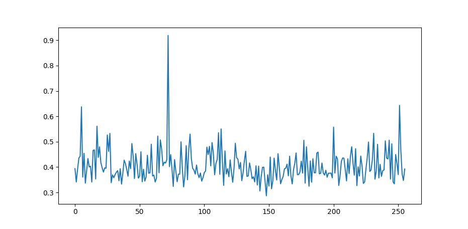
Figure 1: The AES Correlation Coefficients for the first sub-key values

Remember I used the key H4ck3rm4n-l33t42, where H or ASCII 72 is the first sub-key byte. If you used a different key, your plot will most probably look different and there will be a high spike at the ASCII value of your first sub-key.

Well done! We have cracked our first sub-key! Now that we know how to load in our power traces, and we have successfully cracked one of the bytes of the encryption key, we can move on to cracking the entire key.

Automate the cracking process

What will this section cover?

• Automatically selecting which sub-key fits best
• Cracking the entire key

In this section, we are going to expand upon the previous section by automating the cracking process for single bytes and then making the process work on the entire key. Most of what is discussed in this section is quite trivial. If you feel quite comfortable with what was discussed in the previous sections, by all means skip this section and attempt to implement these behaviors yourself. If you get stuck, you can always come back here for a hint.

Where were we?

At the moment, we have code for modeling the AES memory state based power consumption, calculating correlation coefficients between our leakage model and the power traces and a piece of code to plot our results. This is how that all looks together.

import numpy as np
from tqdm import trange

# Modeling the power consumption
########################################
HammingWeightFn = lambda x: bin(x).count('1')

# Precompute Hamming Weight
HammingWeight = [ HammingWeightFn(n) for n in range (0x00, 0xff + 1) ] 

# Rijndael Substitution box
SBox = [
    # 0    1    2    3    4    5    6    7    8    9    a    b    c    d    e    f
    0x63,0x7c,0x77,0x7b,0xf2,0x6b,0x6f,0xc5,0x30,0x01,0x67,0x2b,0xfe,0xd7,0xab,0x76, # 0
    0xca,0x82,0xc9,0x7d,0xfa,0x59,0x47,0xf0,0xad,0xd4,0xa2,0xaf,0x9c,0xa4,0x72,0xc0, # 1
    0xb7,0xfd,0x93,0x26,0x36,0x3f,0xf7,0xcc,0x34,0xa5,0xe5,0xf1,0x71,0xd8,0x31,0x15, # 2
    0x04,0xc7,0x23,0xc3,0x18,0x96,0x05,0x9a,0x07,0x12,0x80,0xe2,0xeb,0x27,0xb2,0x75, # 3
    0x09,0x83,0x2c,0x1a,0x1b,0x6e,0x5a,0xa0,0x52,0x3b,0xd6,0xb3,0x29,0xe3,0x2f,0x84, # 4
    0x53,0xd1,0x00,0xed,0x20,0xfc,0xb1,0x5b,0x6a,0xcb,0xbe,0x39,0x4a,0x4c,0x58,0xcf, # 5
    0xd0,0xef,0xaa,0xfb,0x43,0x4d,0x33,0x85,0x45,0xf9,0x02,0x7f,0x50,0x3c,0x9f,0xa8, # 6
    0x51,0xa3,0x40,0x8f,0x92,0x9d,0x38,0xf5,0xbc,0xb6,0xda,0x21,0x10,0xff,0xf3,0xd2, # 7
    0xcd,0x0c,0x13,0xec,0x5f,0x97,0x44,0x17,0xc4,0xa7,0x7e,0x3d,0x64,0x5d,0x19,0x73, # 8
    0x60,0x81,0x4f,0xdc,0x22,0x2a,0x90,0x88,0x46,0xee,0xb8,0x14,0xde,0x5e,0x0b,0xdb, # 9
    0xe0,0x32,0x3a,0x0a,0x49,0x06,0x24,0x5c,0xc2,0xd3,0xac,0x62,0x91,0x95,0xe4,0x79, # a
    0xe7,0xc8,0x37,0x6d,0x8d,0xd5,0x4e,0xa9,0x6c,0x56,0xf4,0xea,0x65,0x7a,0xae,0x08, # b
    0xba,0x78,0x25,0x2e,0x1c,0xa6,0xb4,0xc6,0xe8,0xdd,0x74,0x1f,0x4b,0xbd,0x8b,0x8a, # c
    0x70,0x3e,0xb5,0x66,0x48,0x03,0xf6,0x0e,0x61,0x35,0x57,0xb9,0x86,0xc1,0x1d,0x9e, # d
    0xe1,0xf8,0x98,0x11,0x69,0xd9,0x8e,0x94,0x9b,0x1e,0x87,0xe9,0xce,0x55,0x28,0xdf, # e
    0x8c,0xa1,0x89,0x0d,0xbf,0xe6,0x42,0x68,0x41,0x99,0x2d,0x0f,0xb0,0x54,0xbb,0x16  # f
]

def hypothetical_power_usage(subkey, plain_text_char):

    # Use the Hamming Weight power usage model
    return HammingWeight[

        # Do a SBox look up of the XOR-ed value
        #
        # Since the Hamming Weight of the SBox value will
        # persist for longer in memory this will make finding the
        # pattern easier. It is also still before the Row Shifting
        # so it doesn't cause trouble.
        SBox [

            # The initial round key XOR-ed with the plain text
            subkey ^ plain_text_char
        ]
    ]
########################################

# Loading our trace data
########################################
import numpy as np

traces = np.load('output/traces.npy')
textins = np.load('output/textins.npy')

num_traces = np.shape(traces)[0]
num_points = np.shape(traces)[1]

########################################

# Pearson correlation
########################################
def covariance(X, Y):
    if len(X) != len(Y):
        print("Lengths are unequal, quiting...")
        quit()

    n = len(X)
    mean_x = np.mean(X, dtype=np.float64)
    mean_y = np.mean(Y, dtype=np.float64)

    return np.sum((X - mean_x) * (Y - mean_y)) / n

def standard_deviation(X):
    n = len(X)
    mean_x = np.mean(X, dtype=np.float64)

    return np.sqrt( np.sum( np.power( (X - mean_x), 2 ) ) / n )

def pearson_correlation_coefficient(X, Y):
    cov = covariance(X, Y)
    sd_x = standard_deviation(X)
    sd_y = standard_deviation(Y)

    return cov / ( sd_x * sd_y ) 
########################################

# Define a function to calculate the Correlation Coefficients for a byte in a
# subkey.
########################################
def calculate_correlation_coefficients(subkey, subkey_index):
    # Declare a numpy for the hypothetical power usage
    hypothetical_power = np.zeros(num_traces)

    for trace_index in range(0, num_traces):
        hypothetical_power[trace_index] = hypothetical_power_usage(
            subkey,
            textins[trace_index][subkey_index]
        )

    # We are going to the determine correlations between each trace point
    # and the hypothetical power usage. This will save all those coefficients
    point_correlation = np.zeros(num_points)

    # Loop through all points and determine their correlation coefficients
    for point_index in range(0, num_points):
        point_correlation[point_index] = pearson_correlation_coefficient(
            hypothetical_power,

            # Look at the individual traces points for every trace
            traces[:, point_index]
        )

    return point_correlation
########################################

# Looping through all possible bytes
########################################
# Save all correlation coefficients
max_correlation_coefficients = np.zeros(256)

# Loop through values this subkey
for subkey in trange(0xff + 1, desc="Attack Subkey"):
    max_correlation_coefficients[subkey] = max(abs(
        calculate_correlation_coefficients(subkey, 0)
    ))
########################################

# Plotting the max_correlation_coefficients
########################################
import matplotlib.pyplot as plt

plt.plot(max_correlation_coefficients)
plt.show()
########################################

Automatically picking the best sub-key guess

Currently, we plot the graph of the maximum correlation coefficients, and we determine from there what the correct option is. We can easily automate this process from the observation that the correct option has the highest correlation coefficient. To select this option, we can use the numpy argmax function.

Replace the code for plotting with the following code.

# Select the element with the highest correlation
best_guess = np.argmax(max_correlation_coefficients)

# Print both the hex value and the ASCII character
print("Best guess: {:02x} or '{}'".format(best_guess, chr(best_guess)))

Now the code will automatically print out the option with the highest correlation coefficient.

Note: If we have done only a few traces and our correlation coefficients are a bit less reliable, we can use np.argsort(...)[::-1] multiple good options. With these options we can then, for example, try to brute force our key with the top 5 best options.

Cracking the entire key

Cracking the entire key is as easy as adding another for loop. This loop will go through all sub-keys and pick the best guess for each sub-key.

This will turn the first piece of code into the second piece of code.

# Looping through all possible bytes
########################################
# Save all correlation coefficients
max_correlation_coefficients = np.zeros(256)

# Loop through values this subkey
for subkey in trange(0xff + 1, desc="Attack Subkey"):
    max_correlation_coefficients[subkey] = max(abs(
        calculate_correlation_coefficients(subkey, 0)
    ))
########################################

# Printing the best guess
########################################
# Select the element with the highest correlation
best_guess = np.argmax(max_correlation_coefficients)

# Print both the hex value and the ASCII character
print("Best guess: {:02x} or '{}'".format(best_guess, chr(best_guess)))
########################################

# Looping through all subkeys
########################################
# The eventual key guess
best_guess = np.zeros(16)

# Loop through all possible subkeys
for subkey_index in trange(16, desc="Subkey Index"):
    # Save all correlation coefficients
    max_correlation_coefficients = np.zeros(256)

    # Loop through values this subkey
    for subkey in range(0x00, 0xff + 1):
        max_correlation_coefficients[subkey] = max(abs(
            calculate_correlation_coefficients(subkey, subkey_index)
        ))
    
    # Save the best guess
    best_guess[subkey_index] = np.argmax(max_correlation_coefficients)
########################################

# Printing the best guess
########################################
print("Best guess:")
for b in best_guess: print("{:02x} ".format(int(b)), end="")
print("")
for b in best_guess: print("{}".format(chr(int(b))), end="")
print("")
########################################

Note: Currently, our code is not very efficient and thus is might take quite a bit of time for it to crack the entire key. This will be optimized in Sidenote: optimizing our code.

This should output the following.

Best guess:
48 34 63 6b 33 72 6d 34 6e 2d 6c 33 33 74 34 32
H4ck3rm4n-l33t42

Correct! This was indeed the key we used to produce our power traces!

We have now successfully cracked the full encryption key from an implementation of AES. We can calculate the best suiting sub-key for each byte of the key and then combine them all together into one by looping over the bytes. Good job!

Sidenote: Optimizing our code

What will this section cover?

• Optimizing the Pearson Correlation Coefficient calculations

As you may have noticed our algorithm is now really slow. This is due to the calculation of Pearson Correlation Coefficients. We can speed this up by a lot if we notice a couple of things.

1. \(\sqrt{a}\sqrt{b}=\sqrt{a b}\). Since square rooting is a very expensive operation, we can optimize the calculation of \(\sigma_x \sigma_y\) from two square root calculations to one.
2. We are recalculating a lot of averages and standard deviations. We can pre-compute these averages and standard deviations and fetch them instead of recomputing them.
3. Since we only care about the maximum correlation coefficient and have no interest in the value itself, we can stop doing any factorization.

In the following code we have created a function which applies these three optimized functions when calculating the correlation coefficients.

point_means = np.mean(traces, axis=0, dtype=np.float64)
point_mean_diff = traces - point_means

point_mean_diff_squared_sum = np.sum(np.power(point_mean_diff, 2), axis=0)

def optimized_calculate_correlation_coefficients(subkey, subkey_index):
    # Declare a numpy for the hypothetical power usage
    hypothetical_power = np.zeros(num_traces)

    for trace_index in range(0, num_traces):
        hypothetical_power[trace_index] = hypothetical_power_usage(
            subkey,
            textins[trace_index][subkey_index]
        )

    hypothetical_power_mean = np.mean(hypothetical_power, dtype=np.float64)
    hypothetical_power_mean_diff = hypothetical_power - hypothetical_power_mean

    hypothetical_power_mean_diff_sum_squared = np.sum(
        np.power(hypothetical_power_mean_diff, 2)
    )

    # We are going to the determine correlations between each trace point
    # and the hypothetical power usage. This will save all those coefficients
    point_correlation = np.zeros(num_points)

    # Loop through all points and determine their correlation coefficients
    for point_index in range(0, num_points):
        point_correlation[point_index] = np.sum(
            hypothetical_power_mean_diff *

            # Look at the individual traces points for every trace
            point_mean_diff[:, point_index]
        ) / np.sqrt(hypothetical_power_mean_diff_sum_squared *
                point_mean_diff_squared_sum[point_index])

    return point_correlation

After optimizing the calculations of the Pearson correlation coefficients, our crack.py script should run a lot faster.

Exercises

Here are some small exercises to verify you understand the material covered.

1. At the following location you can find 3 sets of power traces, can you crack their keys used? You will know when you cracked them.
2. Does the method of correlation power analysis apply to the ChaCha ciphers. Why does it work? Why does it not work?

Compiling your own algorithms

What will this chapter cover?

• Installing toolchains necessary for compiling code for a ChipWhisperer target
• Getting started with the SimpleSerial protocol
• Some useful resources for target algorithms

This walkthrough provides sources for most of the precompiled code you might need. However, in order to some experimentation yourself, you might want to compile some implementation of an algorithm. To do this, there are two things we need: the toolchain to compile to our specific microprocessor architecture and the low-level source code to compile.

The following section will cover how to install the toolchains for the ARM architecture. Following that section, will some things to keep in mind when writing source code for our target. Then, there will be a section on some useful resources concerning ChipWhisperer and algorithms for our target.

Installing Toolchains

What will this section cover?

• Installing the ARM toolchain
• Compiling code

In order to compile code which is usable for our specific microprocessor architecture, we need the toolchain for that specific architecture. As said in the introduction chapter, this walkthrough is using the ChipWhisperer Lite ARM board. Therefore, this section will show how to install the ARM toolchain. For other toolchains, have a look at the ChipWhisperer documentation.

Installing the ARM toolchain

Information on the ARM toolchain can be found here.

Windows and macOS

For Windows and macOS, the installer on the ARM developer website should be enough to install the ARM embedded toolchain.

GNU/Linux

For Debian based systems, including Ubuntu, we can use the following command to install the ARM embedded toolchain.

sudo apt install gcc-arm-none-eabi

For ArchLinux based systems, including Manjaro, we can use the following command to install the ARM embedded toolchain.

sudo pacman -S arm-none-eabi-gcc

Compiling binaries

With the proper toolchain installed, we can compile binaries which are going to be used on ChipWhisperer targets. All SimpleSerial resources mentioned in the Existing resources section contain a Makefile in their root directory. This file provides the computer instructions on how to compile source code. In order to create .hex files — which is the format used to program ChipWhisperer targets — from our source, we can simply run the following command from the root directory of our project, replacing <PLATFORM> with the proper platform.

PLATFORM=<PLATFORM> make

This should create the .hex file in the root directory.

We have now installed the proper toolchain and learned how to compile our own source code. Next up, we want to know how to properly write our source code, so we can best do our measurements.

SimpleSerial protocol

What will this section cover?

• What is the SimpleSerial protocol?
• How to we write source code?
• How do we trigger power traces to start and stop?

In order to run your own algorithms, they first have to be written as source code. The ChipWhisperer framework mostly uses C as the language for the source code of encryption algorithms. This means that any existing C implementation of an encryption algorithms can (most of the time) easily be used on the ChipWhisperer targets. There are a few things to take into account, however. The protocol to send data back and forth between the capture board and the target board, some recommendations when writing or choosing software, and how to start and stop power traces. These will all be covered here.

The SimpleSerial Protocol

In order to send data back and forth between the capture board and the target board and tell the target to start running its algorithm, a specific protocol is often used by ChipWhisperer. It is called the SimpleSerial protocol. It basically explains how to send data to the target (such as keys, plain texts, commands, etc.) and return data back from the target (such as cipher texts, hashes, errors, etc.). Some documentation on the C implementation of the algorithm can be found here. Although, if you use either the official simpleserial-base or the simpleserial-c-template, you almost don't need to worry about the specifics.

Writing / selecting your code

When writing your own algorithms for the ChipWhisperer, it is recommended to either not use the heap or use it sparingly. Most of the boards used as targets by ChipWhisperer don't have a lot of RAM and thus using it sparingly is preferred.

Also, when selecting existing implementations, it is recommended to use embedded hardware or heapless implementations. MBedTLS contains some of the more used encryption algorithms.

Starting / Stopping power traces

On the ChipWhisperer Lite ARM and on many other boards, we use the trigger_high function to start a power trace and the trigger_low to stop a power trace. Both of these functions are available from the hal.h, which is also used by the SimpleSerial protocol.

This means somewhere in your code it should look something like the following.

// ...

trigger_high();

encrypt(...);
// or
decrypt(...);

trigger_low();

// ...

This way your entire encryption or decryption will be captured by the power trace. You can also move the triggers to a specific point of the encryption or decryption, if you want to focus on a specific part of the algorithm.

This should give you most of the information needed to write and/or compile your own implementations of algorithms. The next section will contain some other resources which can help you in this process.

Existing resources

Information on the SimpleSerial protocol

• SimpleSerial README
• ChipWhisperer docs

Templates for source code

• SimpleSerial Base
• SimpleSerial C Template: written for this walkthrough

Specific algorithm implementation with SimpleSerial

• All list of firmware provided by the framework: all the directories starting with simpleserial- can be used.
• SimpleSerial wrapper for NIST Lightweight Cryptography algorithms

Useful C algorithm implementations

• MBedTLS: contains implementations for a lot of the common algorithms
• ChaCha C implementation

Assignment

As a final assignment for this walkthrough, there should a detailed report on some component of power analysis including a demonstration and what effect it has on possible attack vectors. A few categories of what we can look at along with some example topics:

• Breaking an encryption algorithm which is not demonstrated in this walkthrough. Possibly combined with some protections against power analysis. Have a look at the Compiling your own algorithms instructions. Some examples of interesting algorithms are:
  • Breaking the Ed25519 algorithm and providing some protections against power analysis. (Have a look at the following implementation)
  • Breaking ChaCha stream ciphers and providing some protections against power analysis. (Have a look at the following implementation)
• Providing multiple protections on RSA or AES along with analysis of their effectiveness and remaining attack vectors.
• Breaking algorithms by using the data power analysis provides us in new ways.
  • Apply machine learning to the data provides by a power-trace of an encryption algorithm and determine its effectiveness.
  • Look further into optimizing the amount of power traces needed to do a correlation power analysis attack. How many traces can reliably crack a certain algorithm? Can this be improved in some way?

These are just a few examples within the many possible topics. If another creative idea pops up, feel free to give it a shot. The only requirements of the report are a reproducible demonstration and explanation of your method and a description of (remaining) attack vectors through power analysis.

Grading / What will be looked at

There are a few important topics to which is going to be paid attention whilst grading.

Complexity and creativity of method

Most important is the complexity and creativity of your method. These are best formulated by the following two questions:

1. What level of difficulty is your attack vector or method of execution?
2. How much of this method was already pre-done by other people?

This also leads to the point that it is very important to cite sources for your attacks. Any found plagiarism will not be tolerated. If one uses a piece of text, code or method (almost) directly copied or cited from a source, cite that (primary) source. If one adapts a piece of text, code or method from a source, cite as Adapted from ....

Level of explanation and writing

Apart from having a great and creative method, it is also very important to make clear why and why your method was so great and creative. Go into depth on the steps of your method and why those steps help reach the desired result. You can assume that the reader has also followed this walkthrough and albeit has some preliminary knowledge.

Reproducibility

The final important part of your assignment on power analysis is going to be reproducibility. How easy is it for the people checking your assignment to reproduce your method(/results). Is your code readable? Is there some clear documentation on compiling code, executing an attack or installing dependencies? It is not needed to write step-by-step instructions yourself for most of these steps, but it is important to write an overview on installing dependencies (linking to the installation guide of that dependency), compiling instructions (when needed) and attack execution instructions.

Good luck and have fun!