Crack individual key-byte
What will this section cover?
- Loading our saved power traces
- Calculating Pearson correlation coefficients in Python
- Finding the highest Pearson correlation coefficient for a byte of the key used
After creating files containing multiple power traces in the previous section, we can now start analyzing our traces and attempt to crack some bytes with the leakage model we defined in Modeling AES.
So what did we have for our leakage model up until now?
HammingWeightFn = lambda x: bin(x).count('1')

# Precompute Hamming Weight
HammingWeight = [ HammingWeightFn(n) for n in range (0x00, 0xff + 1) ]

# Rijndael Substitution box
SBox = [
    # 0    1    2    3    4    5    6    7    8    9    a    b    c    d    e    f
    0x63,0x7c,0x77,0x7b,0xf2,0x6b,0x6f,0xc5,0x30,0x01,0x67,0x2b,0xfe,0xd7,0xab,0x76, # 0
    0xca,0x82,0xc9,0x7d,0xfa,0x59,0x47,0xf0,0xad,0xd4,0xa2,0xaf,0x9c,0xa4,0x72,0xc0, # 1
    0xb7,0xfd,0x93,0x26,0x36,0x3f,0xf7,0xcc,0x34,0xa5,0xe5,0xf1,0x71,0xd8,0x31,0x15, # 2
    0x04,0xc7,0x23,0xc3,0x18,0x96,0x05,0x9a,0x07,0x12,0x80,0xe2,0xeb,0x27,0xb2,0x75, # 3
    0x09,0x83,0x2c,0x1a,0x1b,0x6e,0x5a,0xa0,0x52,0x3b,0xd6,0xb3,0x29,0xe3,0x2f,0x84, # 4
    0x53,0xd1,0x00,0xed,0x20,0xfc,0xb1,0x5b,0x6a,0xcb,0xbe,0x39,0x4a,0x4c,0x58,0xcf, # 5
    0xd0,0xef,0xaa,0xfb,0x43,0x4d,0x33,0x85,0x45,0xf9,0x02,0x7f,0x50,0x3c,0x9f,0xa8, # 6
    0x51,0xa3,0x40,0x8f,0x92,0x9d,0x38,0xf5,0xbc,0xb6,0xda,0x21,0x10,0xff,0xf3,0xd2, # 7
    0xcd,0x0c,0x13,0xec,0x5f,0x97,0x44,0x17,0xc4,0xa7,0x7e,0x3d,0x64,0x5d,0x19,0x73, # 8
    0x60,0x81,0x4f,0xdc,0x22,0x2a,0x90,0x88,0x46,0xee,0xb8,0x14,0xde,0x5e,0x0b,0xdb, # 9
    0xe0,0x32,0x3a,0x0a,0x49,0x06,0x24,0x5c,0xc2,0xd3,0xac,0x62,0x91,0x95,0xe4,0x79, # a
    0xe7,0xc8,0x37,0x6d,0x8d,0xd5,0x4e,0xa9,0x6c,0x56,0xf4,0xea,0x65,0x7a,0xae,0x08, # b
    0xba,0x78,0x25,0x2e,0x1c,0xa6,0xb4,0xc6,0xe8,0xdd,0x74,0x1f,0x4b,0xbd,0x8b,0x8a, # c
    0x70,0x3e,0xb5,0x66,0x48,0x03,0xf6,0x0e,0x61,0x35,0x57,0xb9,0x86,0xc1,0x1d,0x9e, # d
    0xe1,0xf8,0x98,0x11,0x69,0xd9,0x8e,0x94,0x9b,0x1e,0x87,0xe9,0xce,0x55,0x28,0xdf, # e
    0x8c,0xa1,0x89,0x0d,0xbf,0xe6,0x42,0x68,0x41,0x99,0x2d,0x0f,0xb0,0x54,0xbb,0x16  # f
]

def hypothetical_power_usage(subkey, plain_text_char):

    # Use the Hamming Weight power usage model
    return HammingWeight[

        # Do a SBox look up of the XOR-ed value
        #
        # Since the Hamming Weight of the SBox value will
        # persist for longer in memory this will make finding the
        # pattern easier. It is also still before the Row Shifting
        # so it doesn't cause trouble.
        SBox [

            # The initial round key XOR-ed with the plain text
            subkey ^ plain_text_char
        ]
    ]
We are going to take this as a starting point of a new Python script. This
walkthrough is will refer to that Python file as crack.py. We can thus run
this script from our shell using python3 crack.py.
Loading back in our traces
In order to load the power traces we created in the previous
section, we can add the follow few lines which will load in the
NumPy arrays. The traces here are put into a subfolder called output. If for
any reason making power traces did not work out, or you don't own a
ChipWhisperer board, but you still want to continue, you can download some
pre-made traces from
here.
import numpy as np

traces = np.load('output/traces.npy')
textins = np.load('output/textins.npy')

num_traces = np.shape(traces)[0]
num_points = np.shape(traces)[1]
Now we can use our from the traces variable, we know how many traces we have
(num_traces), and how many points in time we have per trace (num_points).
Implementing Pearson Correlation Coefficients
As explained in the section on Correlation Power Analysis, we are going to be using Pearson Correlation Coefficients to detect whether our power trace is similar to our leakage model. So let us implement Pearson Correlation Coefficients in Python.
def covariance(X, Y):
    if len(X) != len(Y):
        print("Lengths are unequal, quiting...")
        quit()

    n = len(X)
    mean_x = np.mean(X, dtype=np.float64)
    mean_y = np.mean(Y, dtype=np.float64)

    return np.sum((X - mean_x) * (Y - mean_y)) / n

def standard_deviation(X):
    n = len(X)
    mean_x = np.mean(X, dtype=np.float64)

    return np.sqrt( np.sum( np.power( (X - mean_x), 2 ) ) / n )

def pearson_correlation_coefficient(X, Y):
    cov = covariance(X, Y)
    sd_x = standard_deviation(X)
    sd_y = standard_deviation(Y)

    return cov / ( sd_x * sd_y )
Although this code is very inefficient, and does a lot of unnecessary and double calculations, it will serve well for now. We are going to be optimizing this code in Sidenote: optimizing our code.
Cracking a single byte of the key
As explained in Modeling AES, we can — using power analysis — crack the AES key byte by byte. So let us start with a single one. We are going to go through every possibility and see which byte one provides the highest correlation coefficient between the actual power trace and our modeled power usage. The important realization here is that we are doing a correlation between all individual power trace points and the hypothetical power consumption, and we will select the maximum correlation coefficient for all sub-key guesses. This is because we still have no idea where within the power trace the first round actually takes place. If we look at all points of each power trace, the location where the first round takes place should have the highest correlation. We will demonstrate this later on.
from tqdm import trange

def calculate_correlation_coefficients(subkey, subkey_index):
    # Declare a numpy for the hypothetical power usage
    hypothetical_power = np.zeros(num_traces)

    for trace_index in range(0, num_traces):
        hypothetical_power[trace_index] = hypothetical_power_usage(
            subkey,
            textins[trace_index][subkey_index]
        )

    # We are going to the determine correlations between each trace point
    # and the hypothetical power usage. This will save all those coefficients
    point_correlation = np.zeros(num_points)

    # Loop through all points and determine their correlation coefficients
    for point_index in range(0, num_points):
        point_correlation[point_index] = pearson_correlation_coefficient(
            hypothetical_power,

            # Look at the individual traces points for every trace
            traces[:, point_index]
        )

    return point_correlation

# Save all correlation coefficients
max_correlation_coefficients = np.zeros(256)

# Loop through values this subkey
for subkey in trange(0xff + 1, desc="Attack Subkey"):
    max_correlation_coefficients[subkey] = max(abs(
        calculate_correlation_coefficients(subkey, 0)
    ))
This will determine the maximum [correlation coefficients] for all sub-key guesses. If we plot this we get the following graph.
import matplotlib.pyplot as plt

plt.plot(max_correlation_coefficients)
plt.show()
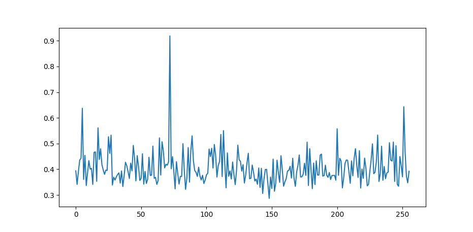
Figure 1: The AES Correlation Coefficients for the first sub-key values
Remember I used the key H4ck3rm4n-l33t42, where H or ASCII 72 is the first
sub-key byte. If you used a different key, your plot will most probably look
different and there will be a high spike at the ASCII value of your first
sub-key.
Well done! We have cracked our first sub-key! Now that we know how to load in our power traces, and we have successfully cracked one of the bytes of the encryption key, we can move on to cracking the entire key.